

![]()
![]()
The BLA R package provides a set of tools to fit
boundary line models to a data set as proposed by Webb (1972). It
includes a suite of methods which have been introduced since the
original manually-drawn boundary lines were proposed. These include
methods based on binning the independent variable, the BOLIDES algorithm
of Schug et al. (1995), quantile regression and the
statistically robust censored bivariate normal model of Milne et
al. (2006). It also provides data exploration methods to check for
outliers and to provide initial evidence for a limiting boundary in data
sets as initial steps before doing boundary line analysis. It includes
functions to determine suitable starting values for boundary line
parameters for estimation by numerical optimization procedures. Learn
more in vignette("Introduction_to_BLA").
Install the current version of the package from CRAN.
install.packages("BLA")The classical situation in which BLA is used is to model
the relationship between some response variable for a biological system
(e.g. the yield of a crop) and a variable which is potentially limiting
on that response (e.g. soil P concentration). The approach is suitable
for large data sets from surveys i.e. cases in which multiple potential
limiting factors occur but are not controlled experimentally. In the
example of crop yield and soil P concentration, one can determine the
largest expected yield for a given soil P concentration value, also
called the boundary pH value. There are various methods to fit the
boundary model in the BLA package, encoded in the functions
blbin(), bolides(), blqr() and
cbvn(). Additionally, the BLA provides
function for initial data exploratory and post-hoc analysis.
The example below uses the censored bivariate normal model,
cbvn(), function to fit the boundary line:
library(BLA)
library(aplpack)
In addition to the BLA, the aplpack package
is loaded which provides the bagplot() function for outlier
detection.
There are three important exploratory steps required prior to fitting
boundary line models when using cbvn(). These include (1)
checking the distribution of the potential limiting and response
variables to access if they fulfill the assumption of normality, (2)
detection of outliers, and (3) the determination of evidence of boundary
existence in a dataset.
The function summastat() can be used for this purpose.
Starting with soil P concentration:
x <- soil$P
summastat(x)
#>         Mean Median Quartile.1 Quartile.3 Variance       SD Skewness
#> [1,] 25.9647     22         16         32 207.0066 14.38772 1.840844
#>      Octile skewness Kurtosis No. outliers
#> [1,]       0.3571429 5.765138           43
From the plots and the summary statistics, the x
variable can not be assumed to be from a normal distribution and hence
requires transformation to fulfill the assumption of normality. You can
do this by taking the natural log of x.
summastat(log(x))
#>          Mean   Median Quartile.1 Quartile.3  Variance        SD  Skewness
#> [1,] 3.126361 3.091042   2.772589   3.465736 0.2556936 0.5056615 0.1297406
#>      Octile skewness    Kurtosis No. outliers
#> [1,]      0.08395839 -0.05372586            0
Normality can now be assumed after transformation. Next, you check
the variable yield.
y <- soil$yield

summastat(y)
#>          Mean  Median Quartile.1 Quartile.3 Variance       SD   Skewness
#> [1,] 9.254813 9.36468   8.203703   10.39477 3.456026 1.859039 -0.4819805
#>      Octile skewness Kurtosis No. outliers
#> [1,]     -0.05793291 1.292635            7
From the plots and the summary statistics, the variable
y can be assumed to be from a normal distribution.
This is done using the bagplot() function from the
aplpack package. Its input is a matrix and
hence we assign the x and y variables to a
matrix data_ur.
  nobs<-length(soil$P)
  data_ur<-matrix(NA,nobs,2)#  create a matrix: bagplot inputs data as a matrix
  data_ur[,1]<-log(soil$P)
  data_ur[,2]<-soil$yield

  bag<-bagplot(data_ur,create.plot = F ) # bagplot identifies outliers

data<-rbind(bag$pxy.bag,bag$pxy.outer) # new excludes bivariate outliersThis is done using the function expl_boundary()
  x <- data[,1]
  y <- data[,2]

  expl_boundary(x,y,10,1000)
#> Note: This function might take longer to execute when running a large number of simulations.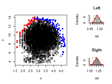
#>     Index Section    value
#> 1      sd    Left 1.045711
#> 2      sd   Right 1.115379
#> 3 Mean sd    Left 1.132397
#> 4 Mean sd   Right 1.201709
#> 5 p_value    Left 0.037000
#> 6 p_value   Right 0.041000
The p-values in the left and right sections are less than 0.05, indicating evidence of boundary existence. This justifies the fitting of a boundary line model to the dataset.
Based on the structure of the data at the upper edge, a trapezium
model can be fitted. Take note that any other model of your choice that
is biologically plausible can be fitted. Below is an example of how you
can use the cbvn() function to fit the boundary line.
It arguments include (1) a dataframe,data, containing
the x and y variables, (2) a vector of initial
start values for the optimization that includes the
parameters of the boundary model and for the distribution
(i.e. mean(x), mean(y), sd(x),
sd(y) and cor(x,y)), and (3) the measurement
error value, sigh, for the response variable. The rest of
the inputs are related to the plot features as in the function
plot() from base R.
The start values for the preferred model can be determined using the
startValues() function. Set the argument model
to the desired model e.g. model="trapezium", run the
function and click on the plot of y against x,
the points that make up the structure of the model at the upper edges of
the data scatter.
plot(data)

startValues("trapezium")
Using the obtained values for the model, create a vector of start values.
data<-data.frame(x,y)
start<-c(4,3,13.6, 35,-5,3,9,0.50,1.9,0.05) # initial start values for optimization

model <- cbvn(data, start = start, model = "trapezium", sigh=0.7,
                 xlab = expression("Soil P"), ylab = expression("Yield/ t ha"^-1),
                 pch = 16, plot = TRUE, col = "grey40", cex = 0.6)
model
#> $Model
#> [1] "trapezium"
#>
#> $Equation
#> [1] y = min (β₁ + β₂x, β₀, β₃ + β₄x)
#>
#> $Parameters
#>          Estimate Standard error
#> β₁     4.29795522    1.035391840
#> β₂     3.23397375    0.460850826
#> β₀    13.15187257    0.206656034
#> β₃    33.17267393    1.693458789
#> β₄    -5.22857503    0.393758941
#> mux    3.12597270    0.006451086
#> muy    9.30482617    0.022879293
#> sdx    0.50053107    0.004561474
#> sdy    1.60754420    0.018448808
#> rcorr  0.04150832    0.014806076
#>
#> $AIC
#>
#> mvn 32429.55
#> BL  32391.07
The output gives the name of model fitted which is a “trapezium” in the case, its equation form, its parameters (the first 5 rows of the Parameters) and corresponding standard errors, and the AIC values for the boundary model, BL, and a corresponding multivariate normal model, mvn. Since the AIC for the BL is smaller than mvn, the boundary line model is appropriate.
The boundary yield given the soil P concentration for each data point
can be predicted using the function predictBL() :
P_values <- log(soil$P)
P_values[is.na(x)] <- mean(x, na.rm = TRUE) # replace missing values with mean pH
predicted_yield <- predictBL(model, P_values)


head(predicted_yield) # predicted yield for the first six farms
#> [1] 11.74445 11.40372 11.74445 11.40372 11.40372 12.33408
The critical P value is the point beyond which yield increase is not expected. You can calculate it from the model parameters as follows:
intercept <- model$Parameters[1]
slope <- model$Parameters[2]
plateau <- model$Parameters[3]

critical_P <- (plateau - intercept) / slope

print(exp(critical_P))# results are in mg/l
#> [1] 15.45268
Other boundary line post-hoc analysis procedures can be conducted.
For more information, See
vignette("Censored_bivariate_normal_model") and
vignette("Introduction_to_BLA").
Milne, A. E., Wheeler, H. C., & Lark, R. M. (2006). On testing biological data for the presence of a boundary. Annals of Applied Biology, 149 , 213-222. https://doi.org/10.1111/j.1744-7348.2006.00085.x
Schnug, E., Heym, J. M., & Murphy, D. P. L. (1995). Boundary line determination technique (bolides). In P. C. Robert, R. H. Rust, & W. E. Larson (Eds.), site specific management for agricultural systems (p. 899-908). Wiley Online Library. https://doi.org/10.2134/1995.site-specificmanagement.c66
Webb, R. A. (1972). Use of the boundary line in analysis of biological data. Journal of Horticultural Science, 47, 309–319. https://doi.org/10.1080/00221589.1972.11514472